While the Fed’s 75bps hike on Wednesday 21st was in line with expectations, the market had priced in a 100 bps hike for the SNB. In this sense the 75bps announcement came as a dovish surprise, even though this still is the biggest SNB rate increase in more than 20 years.

While the SNB explicitly did not rule out further hikes in December and, if necessary, forex market intervention in the interim, it is noteworthy to what extent governor Thomas Jordan emphasized the role of international spillovers through the hiking of other central banks and the role of transitory inflation pressures in his opening statement and the subsequent media Q&A.

In this context, it may therefore be interesting to widen the perspective to the international level to take stock where we stand in what one might call the “global tightening cycle” and how we got here. As “global tightening cycle” I define the current thrive of virtually all major central banks in advanced economies (except maybe Japan) to tighten monetary policy in often quite dramatic (50-75bps) increments in order to fight global inflation pressure.

The “global tightening cycle”: a shift from “Camp Transitory” to “Camp Permanent”

Roughly a year ago, most AE central bankers were firmly in what I want to call “camp transitory”. The tenet of “camp transitory” was that quickly rising inflation would come down again largely on its own because it reflected a combination of several, well, transitory factors: a) basis effects as prices had declined during the Covid crisis and were now increasing again b) transient supply bottlenecks amidst a recovery that affected different sectors at different speeds leading to, c), large relative sectoral price changes and, d), an increase in energy prices due to increased demand as the global economy recovered.

Also, because the factors above, and in particular b) and d), are global phenomena, there was a perception that there was little domestic monetary policy could do — always provided that inflation expectations would stay anchored.

Over the last year, most AE central bankers seem to have switched to “camp permanent” though, and so, it appears, for good reason:
Global intermediate input supply bottle necks proved more persistent than many expected (largely due to China’s continued zero-COVID policy) while Russia’s invasion of Ukraine and the ensuing sanctions drove up energy and food prices. In the US, an additional factor was the passing of another round of gigantic fiscal stimulus in the form of the (in)aptly named “inflation reduction act”. Most importantly, all of these shocks started to be reflected in a persistent upward drift of inflation expectations.

A textbook view on permanent and transitory supply shocks

Except for the US fiscal stimulus, all of the above shocks can be considered as “supply-side” and it may therefore be instructive to look at what our undergraduate text-book macroeconomics — in the form of the venerable AS-AD model— has to say about transitory and permanent supply shocks. NOTE: if you can’t be bothered to read this (you may be forgiven), then just go to “TLDR” below for the main take aways.

The graph below illustrates permanent and transitory supply shocks in the AS-AD model. The upper panel reflects a permanent supply shock, the lower panel a transitory supply shock. In both panels, the economy is initially at equilibrium at point A where the short-run aggregate supply curve (SAS), the lon-run aggregate supply curve LAS and the aggregate demand curve AD all intersect. At point A inflation is at its long-run expected level  π^e, output on its long-run trend Yⁿ and unemployment at its natural rate.

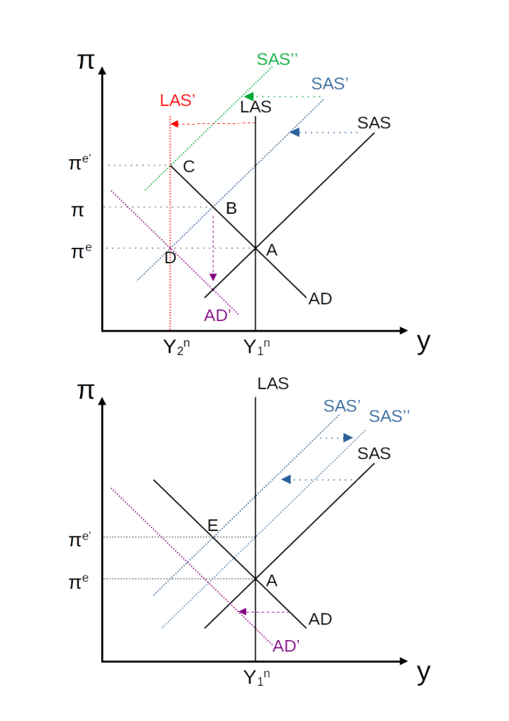
Consider the permanent supply shock in the upper panel first. A permanent supply shock reduces the productive capacity of the economy and therefore shifts the LAS curve left, to LAS’. Think of the SAS-curve as being nailed to the LAS-curve at the point where π=π^e so that it shifts together with LAS as Y₁ⁿ drops to Y₂ⁿ to the new short-run supply curve SAS’.

As a result, there is a new short-run equilibrium with higher inflation and lower output at point B. But of course that’s not the end of it. As firms and households observe inflation is higher than they expected, they will revise their expectations upwards. Recall that the new SAS’ curve intersects the LAS’ curve where π=π^e. This means that the SAS’ curve shifts further upwards if inflation expectations increase, leading to even higher inflation and even lower output. Where does it all end? Well, in point C, where we have permanently higher inflation and permanently lower output.

So what should the central bank do? The answer is: it should act decisively to avoid that people adjust their expectations upward . Ideally, it would nip any increase in inflation expectations in the bud (i.e. avoid any “second round effects”) by shifting the AD curve downward to AD’, so that it intersects the other two curves at point D.

So far, so textbook. But it is worth noting what this means: in this setting there is no cost in terms of additional lost output to decisive monetary tightening. The reason is that in the medium-term, irrespective of whether the central bank acts or not, the economy will have the new, lower trend output Y₂ⁿ anyway. There is just the choice between a permanently high-inflation equilibrium (C) or a low-inflation equilibrium (D). In that sense, in this permanent supply shock scenario the central bank can always engineer a “soft landing”, i.e. reduce inflation without a recession (defined as output being below its long-term / trend level). The crux of the matter however is: it does not feel like a soft landing at all. The transition from A to C or D comes with a decisive reduction in incomes and living standards and an increase in the natural rate of unemployment. It will not feel like we are in a boom (relative to our new normal at Y₂ⁿ)  but in a deep recession that lasts forever….

Now consider a transitory negative supply shock (lower panel). Transitory in this model means that the LAS curve does not move because trend output is not changed. But the short-run aggretate supply curve SAS moves left. Recall why this happens: the SAS is essentially the famous Phillips-curve in disguise and it says that firms are willing to temporarily supply more output (and hire more labor, lowering unemployment) if prices (and thus inflation) exceed their expected level. This happens because wages and many other input costs are usually sluggish and their prices are set based on previous expectations. Hence, it is profitable to hire more labor and produce more output while wages are still fixed at old levels (predicated on previous expectations of costs of living). This explains the upward slope of the SAS.

Now, with a temporary negative supply shock (e.g. rising gas prices), firms will want to supply less output for any given inflation surprise, leading to the leftward shift to the new short run supply curve SAS’. The result is higher inflation and a recession in point E.
But what should the central bank do here? Recall that by tightening policy it would shift the AD curve downwards (say to AD’) which would lower inflation but also deepen the recession. In fact, if the shock to SAS is temporary, the best option is to do nothing. If the gas price drops again (or if firms find good subsitutes for gas), then the SAS’ curve will shift right again. Note that this will generally be gradual even if the underlying transitory shock is already gone. Why? Well, the reason is again inflation expectations and the fact that (in the absence of temporary supply shocks) LAS and SAS will intersect at π=π^e. Hence, if people observe inflation being higher than they expected, they will revise these expectations upwards, so that (even with the original supply shock gone), the SAS curve will not immediately shift back again but will only gradually shift back (see e.g. SAS”).

Interestingly, that implies that inflation expectations will stay elevated (relative to where we started at point A) for a while. But with the short-run supply curve at SAS” , actual inflation will start to undershoot people’s expectations, leading them to gradually revise them downwards and taking us back to point A.

TLDR: So, which scenario are we in? Permanent or transitory? Of course that is exactly the question that central bankers have to answer. As the shocks happen, we just don’t know. In both scenarios inflation expectations will initially increase so telling the two apart in real time will not work! But the policy recommendations could not be more different: if the shock is permanent, aggressive tightening is the clear-cut recommendation. If the shock is transitory, not doing anything is the best a central bank can do. This explains why AE central banks were initially hesitant to act on early signs of increasing inflation and it may also help understand their highly synchronized move to sharp tightening as soon as evidence of de-anchoring of inflation expectations became more salient — the “global tightening cycle”.

Shocks may be less persistent than we thought

Fortunately, recent data give us some clues: Oil prices have already fallen to well below 100 dollar a barrel from their peaks in the first two quarters of 2022. Forward gas prices are down by half for the spring on current spot prices which (even allowing for seasonal peaks in price during winter) is considerable. Inflation expectations in the U.S. have peaked already. Food exports from Ukraine are slowly resuming…

All this suggests that there is a considerable temporary component to all these negative supply shocks.

But there is a more fundamental issue that concerns the very structure of our economies: How persistent a supply shock eventually turns out to be is ultimately also determined by how quickly the economy can substitute away from expensive inputs.

And here the evidence is quite encouraging as well. Germany for example is highly dependent on gas imports and industry lobbyists and politicians were and still are predicting the worst. However, a group of German economists around Ben Moll at LSE and Christian Bayer at Uni Bonn have shown quite persuasively that the ability of the economy as a whole to subsitute this apparently indispensable input has been systematically underestimated. Recent empirical evidence suggests that Germany was able to reduce gas consumption by 20 percent over a year without a reduction output and, so far, without an increase in unemployment. This does not mean that there will be no recession, but it means that it (the recession, and with it, inflation) may be more transitory (and possibly less deep) than many have thought.

All this suggests that negative supply factors driving inflation at the global level are already mitigating, providing a good reason for the SNB to tread relatively carefully on its rate rises while still sending a determined signal of being prepared to act if inflationary pressures really turn out to be more persistent than expected.

Importance of international spillovers

In trade-weighted terms, the franc has appreciated by arond 7% since mid-year which gives a considerable buffer that shields Swiss consumer prices from inflation elsewhere. That’s partly due to the previous Swiss hikes but also due to the appreciation that the Swiss franc as a safe haven currency typically sees during times of crisis. This is a first way in which global factors may also dampen inflation here in Switzerland

Add to this another good reason for the SNB to stay its hand: the “hikes of others” (most notably the Fed) are already doing a lot of the work. Global tightening is already mitigating demand for Swiss exports in the rest of the world while the real bilateral exchange rate vis-à-vis the euro area (from which we get most. of our imports of consumption goods) has appreciated considerably. Hence, keeping interest rate differentials vis-à-vis the dollar and euro constant by setting them to the levels at which they were before the recent ECB and Fed rate hikes (by also doing a 75bps) made sense.

Maurice Obstfeld has just recently warned that the current hiking cycle has neglected the powerful international spillover effects from rate increases and that central bankers just looking at domestic conditions might well do too much of a good thing.
The SNB seems to have been heeding Obstfeld’s point in its decision this morning. With Swiss inflation standing at less than half of what it is in the US and the euro area, it could afford to wait all while keeping all options on the table.